Definition (Distance Function/Metric): A distance function, also known as a metric, is a function \(d: M \times M \rightarrow \mathbb{R}\), where \(M\) is a set, satisfying the following:
\(d(x, y) \geq 0 \forall x, y \in M\) (Non-negativity),
Definition (Euclidean distance on\(\mathbb{R}^d\)): The Euclidean distance between two points \(\mathbf{x}, \mathbf{y} \in \mathbb{R}^d\) is defined as follows: \[
d_E(\mathbf{x}, \mathbf{y}) = \| \mathbf{x} - \mathbf{y} \| = \sqrt{\sum\limits_{j=1}^d (x_j - y_j)^2}.
\] The Euclidean distance is one of the most basic and most useful distance functions that you are probably already familiar with. It can be calculated in any finite dimension \(p\) and has a very intuitive interpretation as the length of the line segment between any two observations.
Example: The Euclidean distance on \(\mathbb{R}^d\) is a valid distance function. Let’s prove this:
1. Non-negativity:
Since \((x_j - y_j)^2 \geq 0\) for all \(j\), we have \(\sum_{j=1}^d (x_j - y_j)^2 \geq 0\). Taking the square root preserves non-negativity, so \(d_E(\mathbf{x}, \mathbf{y}) = \sqrt{\sum_{j=1}^d (x_j - y_j)^2} \geq 0\).
\((\Rightarrow)\) If \(d_E(\mathbf{x}, \mathbf{y}) = 0\), then \(\sqrt{\sum_{j=1}^d (x_j - y_j)^2} = 0\), which implies \(\sum_{j=1}^d (x_j - y_j)^2 = 0\). Since each term \((x_j - y_j)^2 \geq 0\) and their sum is zero, we must have \((x_j - y_j)^2 = 0\) for all \(j\), therefore \(x_j = y_j \forall j \in \{1, \ldots, d\}\), so \(\mathbf{x} = \mathbf{y}\).
\((\Leftarrow)\) If \(\mathbf{x} = \mathbf{y}\), then \(x_j = y_j\) for all \(j\), so \(d_E(\mathbf{x}, \mathbf{y}) = \sqrt{\sum_{j=1}^d 0^2} = 0\).
4. Triangle inequality:
We need to show \(d_E(\mathbf{x}, \mathbf{z}) \leq d_E(\mathbf{x}, \mathbf{y}) + d_E(\mathbf{y}, \mathbf{z})\), or equivalently: \[\|\mathbf{x} - \mathbf{z}\| \leq \|\mathbf{x} - \mathbf{y}\| + \|\mathbf{y} - \mathbf{z}\|.\]
Note that \(\mathbf{x} - \mathbf{z} = (\mathbf{x} - \mathbf{y}) + (\mathbf{y} - \mathbf{z})\). By the Cauchy-Schwarz inequality and properties of norms in \(\mathbb{R}^d\), we have: \[\|\mathbf{x} - \mathbf{z}\| = \|(\mathbf{x} - \mathbf{y}) + (\mathbf{y} - \mathbf{z})\| \leq \|\mathbf{x} - \mathbf{y}\| + \|\mathbf{y} - \mathbf{z}\|.\]
This is the standard triangle inequality for the Euclidean norm. \(\square\)
The Manhattan distance
Definition (Manhattan distance on\(\mathbb{R}^d\)): The Manhattan distance (also known as taxicab, city block, or rectilinear distance) between two points \(\mathbf{x}, \mathbf{y} \in \mathbb{R}^d\) is defined as follows: \[
d_T(\mathbf{x}, \mathbf{y}) = \| \mathbf{x} - \mathbf{y} \|_T = \sum\limits_{j=1}^d \lvert x_j - y_j\rvert.
\] The Manhattan distance makes use of the so-called Manhattan geometry, where the distance between any two points is defined as the sum of the absolute differences of their Cartesian coordinates.
💡 Fun fact
The reason it’s called the “Manhattan”, “taxicab”, or “city block” distance is because of the famous borough of Manhattan in New York City, which is planned with a rectangular grid of streets, meaning that a taxicab can only travel along grid directions.
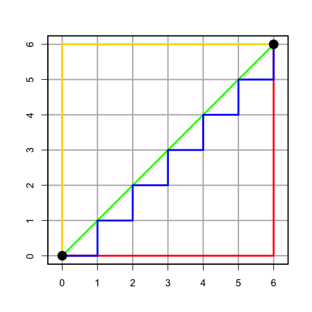
Note🤔 Quiz: Which of the following line colours in the Figure illustrate the Euclidean distance between \((0, 0)\) and \((6, 6)\) and which illustrate the Manhattan distance?
A. Euclidean: Yellow, Manhattan: Red, Blue, Green
B. Euclidean: Blue, Red, Manhattan: Yellow, Green
C. Euclidean: Blue, Red, Yellow Manhattan: Green
D. Euclidean: Green, Manhattan: Blue, Red Yellow
Show Answer
Error 404: Answer not found.
But seriously, think about it this way; if each square is a building and the lines are the roads, which of these routes could a taxi take? 🚕
The Minkowski distance
Definition (Minkowski distance on\(\mathbb{R}^d\)): The Minkowski distance between two points \(\mathbf{x}, \mathbf{y} \in \mathbb{R}^d\) is defined as follows: \[
d_M(\mathbf{x}, \mathbf{y}) = \| \mathbf{x} - \mathbf{y} \|_M = \left(\sum\limits_{j=1}^d \lvert x_j - y_j\rvert^p\right)^{\frac{1}{p}}, \quad p \geq 1.
\] You can see that the Minkowski distance is the Manhattan distance for \(p=1\) and the Euclidean distance for \(p=2\). The Minkowski distance is a generalisation of both!
💡 Fun fact
When \(p \rightarrow \infty\), the Minkowski distance becomes equivalent to: \[
\lim\limits_{p \rightarrow \infty} \left( \sum\limits_{j=1}^d \lvert x_j - y_j \rvert^p \right)^{\frac{1}{p}} = \max\limits_{1 \leq j \leq d} \lvert x_j - y_j \rvert,
\] which is known as the Chebyshev distance; can you prove this result?
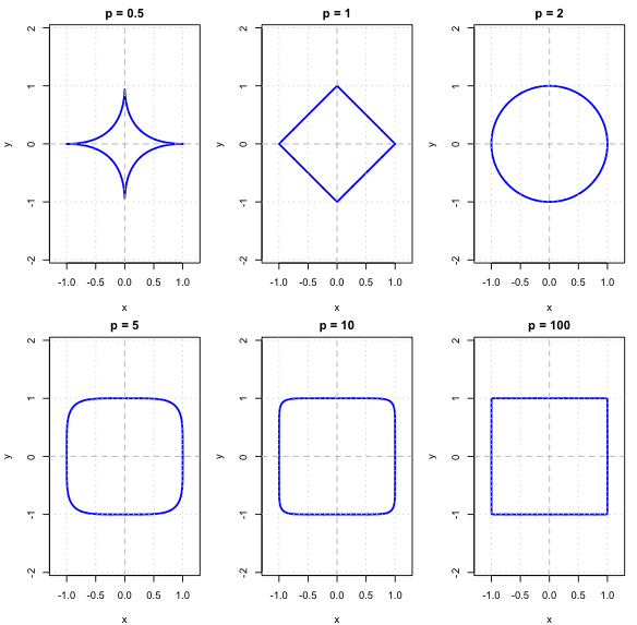
The Figure below displays the “unit circles” for the Minkowski distance with varying \(p\). Notice that \(p = 0.5\) is also included; this does not define a proper distance function.
Unit circles for the Minkowski distance with varying p values. Source: Author’s own work.
Dissimilarities vs. Distances
Definition (Dissimilarity Function): A dissimilarity is a function \(d: M \times M \rightarrow \mathbb{R}\), where \(M\) is a set, satisfying the following:
\(d(x, y) \geq 0 \forall x, y \in M\) (Non-negativity),
A dissimilarity function relaxes the requirement for the triangle inequality to hold. This is precisely what distinguishes a dissimilarity from a distance function. Therefore, all distance functions are valid dissimilarity functions. However, the opposite direction is not always true!
Example: The Minkowski function with \(p=0.5\) is a dissimilarity function but not a distance function.
Let’s prove this together; firstly, we note that the 3 shared conditions (non-negativity, symmetry, indiscernibles) are trivially true. We only need to check for the triangle inequality.
Let us take \(\mathbf{x} = (0, 0)^\top\), \(\mathbf{y} = (1, 1)^\top\) and \(\mathbf{z} = (0, 1)^\top\). Then: \[
\begin{align}
d_M(\mathbf{x}, \mathbf{y}) = \left(\sum\limits_{j=1}^d \lvert x_j - y_j\rvert^\frac{1}{2}\right)^{2} = (1 + 1)^2 = 4,\\
d_M(\mathbf{x}, \mathbf{z}) = \left(\sum\limits_{j=1}^d \lvert x_j - y_j\rvert^\frac{1}{2}\right)^{2} = (0 + 1)^2 = 1,\\
d_M(\mathbf{y}, \mathbf{z}) = \left(\sum\limits_{j=1}^d \lvert x_j - y_j\rvert^\frac{1}{2}\right)^{2} = (0 + 1)^2 = 1.
\end{align}
\] Therefore, \(d_M(\mathbf{x}, \mathbf{y}) > d_M(\mathbf{x}, \mathbf{z}) + d_M(\mathbf{y}, \mathbf{z})\), which means that the triangle inequality does not hold. Therefore, the Minkowski distance with \(p = 0.5\) is a dissimilarity but not a distance function. \(\square\)
💡 Fun fact
The Minkowski function with \(0 < p < 1\) is a dissimilarity function but not a proper metric (can you prove this?), whereas for \(p \geq 1\), it is a distance function.
Note🤔 Quiz: Some of the following functions are valid distance functions, while others are dissimilarities but not distances. Which of these are distance functions?
A. \(d(\mathbf{x}, \mathbf{y}) = \sum\limits_{j=1}^d \frac{\lvert x_j - y_j \rvert}{\lvert x_j \rvert + \lvert y_j \rvert}\).
B. \(d(\mathbf{x}, \mathbf{y}) = 1 - \frac{\mathbf{x} \cdot \mathbf{y}}{\| \mathbf{x} \| \| \mathbf{y} \|}\).
C. \(d(\mathbf{x}, \mathbf{y}) = \sum\limits_{j=1}^d \mathbb{I}\{ x_j \neq y_j\}\) for binary vectors \(\mathbf{x}, \mathbf{y}\).
D. \(d(\mathbf{x}, \mathbf{y}) = \min\limits_{1 \leq j \leq d} \lvert x_j - y_j \rvert\).
E. \(d(\mathbf{x}, \mathbf{y}) = \sqrt{\left(\mathbf{x} - \mathbf{y}\right)^\top \mathbf{S}^{-1}\left(\mathbf{x} - \mathbf{y}\right)}\), where \(\mathbf{S} \in \mathbb{R}^{d \times d}\) is symmetric positive definite.
Show Answer
This answer is currently in an entangled quantum state with your understanding.
Observe it too soon and you’ll collapse the learning wave function. ⚛️
Similarities
Definition (Similarity Function): Given a dissimilarity function \(d: M \times M \rightarrow \mathbb{R}\), a similarity function is a defined as \(s : M \times M \rightarrow [0, 1]\) with \(s(\mathbf{x}, \mathbf{y}) = f(d(\mathbf{x}, \mathbf{y}))\), where \(f:[0, \infty) \rightarrow [0, 1]\) is a decreasing function with \(f(0) = 1\) and \(\lim\limits_{t \rightarrow \infty} f(t) = 0\).
Example: Let \(f(t) = \exp\left( - \frac{t^2}{2\gamma^2} \right)\) for \(\gamma > 0\). The following function is a valid similarity: \[
s(\mathbf{x}, \mathbf{y}) = f(d_E(\mathbf{x}, \mathbf{y})) = \exp\left\{ - \frac{\sum\limits_{j=1}^d (x_j - y_j)^2}{2\gamma^2} \right\}, \gamma > 0, \mathbf{x}, \mathbf{y} \in \mathbb{R}^d.
\] This is also known as the Gaussian kernel or Radial Basis Function (RBF) kernel(you do not need to know what a kernel is at this point, but it is a very useful concept in machine learning).
If I give you the answer now, what’s the similarity between actual learning and just reading answers?
Exactly: \(f(\text{similarity}) = 0\). Check back after class! 😉
Computing distances in R
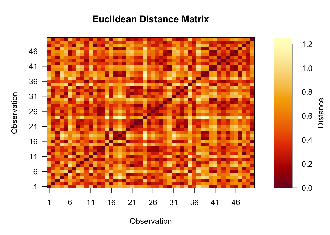
The dist function provides an easy and quick way of computing distances (or dissimilarities) in R. The output is a distance/dissimilarity matrix, which you can also visualise! Below is a toy example with 50 randomly generated 2-dimensional vectors, where each component is drawn from a standard Uniform distribution.
# Set the seed for reproducibilityset.seed(123)# Generate 50 2D random vectors = 100 standard uniform values# Store in a 50 x 2 matrixX <-matrix(data =runif(n =100, min =0, max =1),nrow =50,ncol =2)dist_mat <-dist(x = X, method ="euclidean")dist_matrix <-as.matrix(dist_mat, nrow =nrow(X), ncol =nrow(X))# Create layout with space for legendlayout(matrix(c(1, 2), nrow =1), widths =c(4, 1))# Adjust margins for main plot (bottom, left, top, right)par(mar =c(5, 5, 4, 1))# Main plot with custom paletten_colors <-256colors <-hcl.colors(n_colors, palette ="YlOrRd")image(x =1:nrow(dist_matrix),y =1:ncol(dist_matrix),z = dist_matrix,col = colors,xlab ="Observation",ylab ="Observation",main ="Euclidean Distance Matrix",axes =FALSE)axis(1, at =seq(1, 50, by =5))axis(2, at =seq(1, 50, by =5), las =1)box()# Color bar legend with matching colorspar(mar =c(5, 1, 4, 4))legend_values <-seq(min(dist_matrix), max(dist_matrix), length.out = n_colors)image(x =1, y = legend_values, z =matrix(legend_values, nrow =1),col = colors, axes =FALSE, xlab ="", ylab ="")axis(4, las =1)mtext("Distance", side =4, line =2.5)
The image function produces a heat map but notice how it requires an argument of class matrix. Therefore, we make sure to convert our distance matrix object to a matrix object and specify the number of rows and columns, which has to be equal to \(n\).
💡 Fun fact
The dist function supports several distance metrics. Explore its documentation by typing ?dist on the console and see what other distance functions can be implemented, besides the Euclidean. How would you compute the dissimilarity matrix for a dissimilarity function that is not included in the documentation?
🚀 Time to practice!
Generate some synthetic data (e.g. by sampling from a uniform or a Normal distribution) and use the dist function with any distance function of your choice. Repeat this process but keep increasing the number of dimensions. What do you observe?
(Hint: Use the image function to visualise the distance matrix each time).
Key takeaways
Clustering algorithms use distances, dissimilarities, or similarities to assign objects into groups.
Points with low pairwise distances/dissimilarities are commonly assigned in the same cluster, whereas highly distant/dissimilar points are in distinct clusters.
All distances are dissimilarities but not the other way round.
The triangle inequality is what makes a dissimilarity function a proper distance function.
Large distance/dissimilarity \(\implies\) low similarity, while low distance/dissimilarity \(\implies\) high similarity.
The dist function in R can be used for computing a distance matrix.